Variational Auto-encoders

• Previously, my blog post spoke about generative adversarial networks, and how they work to create new samples of data from a learned distribution.
• In this post, we will look at another class of generative models based on auto-encoders, called “variational” auto-encoders.

What are Auto-encoders?

• Before diving into the details of what variational auto-encoders are, let us first understand what an auto-encoder does. An auto-encoder is a two-stage network architecture consisting of an encoder and a decoder. This is as shown in the image below. A bottleneck is at the interface of the encoder and decoder.

• You might be wondering what the point of such a network that takes an image and spits out the same image might be. It is not the output that we are interested in, but the bottleneck in between. This bottleneck is like a lower-dimensional compact code used to represent the input image. This code is valuable and find many uses in computer graphics and image compression. This low dimensional representation is also called the latent space representation.
• Auto-encoders are trained to minimize something called a reconstruction loss. The reconstruction loss, as the name suggests is the error between the reconstructed image at the output and the original image that you started out with.
• The reason auto-encoders have the word “auto” in them is because they automatically are able to reconstruct themselves.
• If the encoder has tunable parameters \theta and the decoder has parameters \phi, then the objective of the autoencoder is to find the optimal set of parameters for both networks that can minimize the error between the original and the reconstructed image, typically represented as a reconstruction loss. This reconstruction loss is as shown in the image below (where x_i is the ith image in the dataset):

• The encoder network today is usually a Convolutional neural network (CNN). The decoder is also a CNN, but the layers perform image up-sampling rather than down-sampling.
• Also note that there are no external labels being used here, as would be the case in object classification and detection. Sometimes, auto-encoders are useful to initiate a supervised learning problem as well. Once the latent space representation has been learned properly, we can throw away the decoder part of the network, and use the latent space representation to initialize a classification model.
• However, a downside of auto-encoders is that, they cannot be used to generate new images that it has never seen before. This is because it is being penalized on how closely it can reconstruct the input data. This naturally prohibits it from learning any variation from the original data. However, the latent space representation is nevertheless a useful ingredient. The question is – can we somehow tweak the network to use this latent representation to learn new data?

Enter Variational Autoencoders!

• In a nutshell, variational autoencoders are a probabilistic spin on autoencoders.
• Let’s start by assuming that the training data x is constructed from some underlying latent representation vectors. Each element of z is capturing the notion of features that make up our training data. For example, if our training data is a set of faces, elements of z can be representative of features like the relative positioning of eye-brows in the face or the orientation of the face.
• In a generative model, we will choose the individual elements of z by sampling from something like a Gaussian distribution, and generate the image x, based on this distribution. This is essentially saying that we are generating data x conditioned on our choice of z.
• Obviously generating data from some latent representation is not trivial, and we need something that has a lot of parameters. Neural networks are complex and have a lot of tunable parameters. More formally, we want a network to learn parameters \theta^{*} such that it generates training data x given z. This network is the new decoder with a twist – it can generate new data!
• The choice of the distribution is reasonable as it can be used to represent the extent of some elements in z. Going from the example mentioned earlier, this can be things such as the how much smile needs to be there on the face a person or how much the person’s head must be tilted.
• How would we train this network?
  • We can use something called “maximum likelihood”.
  • The intuition behind this is simple – “if the model is likely to produce training set samples, it is also likely to produce similar samples, and unlikely to produce dissimilar ones”.
  • We want to tweak the parameters of our model \theta^* that maximizes this likelihood as shown here:
  • Here, the distribution P(z) is a Gaussian distribution as mentioned earlier (and Gaussians are parameterized by some mean and covariance).
  • Initially during training, the outputs we get will look nothing like the training data. However, on using a Gaussian, it is possible to use something like Gradient descent to make P(X) more likely.
  • Computing the above integral is not tractable for every possible z given only a decoder. However, in combination with an encoder, which can estimate P(z|x), we will get a lower bound for the above integral. This makes it tractable, and something we can optimize.
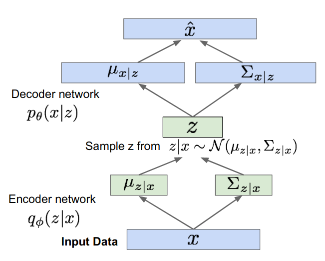
• Given the probabilistic twist to autoencoders, the variational autoencoders will do as shown in the image below. The encoder having parameters \phi which will estimate some distribution of z, instead of some absolute value. Since this distribution is assumed to be Gaussian, it will output some mean and covariance for z given the input data.

• Similarly, the decoder network (having parameters \theta) will take in these probabilities of z, and will output likelihood outputs of x having some mean \mu_{x|z} and covariance \Sigma_{x|z}.
• Sometimes, encoder network in the context of VAEs are also called recognition/inference networks, and decoder is called the “generation” networks.

Training Autoencoders

• First we pass a mini-batch of input images into our encoder, which will give out a distribution of z, given x.
• Sample some z from the distribution that was spit out by the encoder.
• Pass this sampled z through the decoder network, and from the decoder network get the output for the distribution for x given z. Finally, we can sample x given z from this distribution, which will generate a sample output.
• The loss term will try to maximize the likelihood of the generated output being close to the training data. This loss involves something called a KL divergence term (which measure the distance between two distributions). For brevity, I will not go over the mathematical derivation of this loss function.
• For every batch of input, we will compute this forward pass. All the elements in the loss are differentiable, so we then backpropogate our gradients to update the parameters of the encoder and decoder networks to maximize the likelihood of our training data.

What’s next?

• Once we’ve trained our VAE, we can use just the decoder network to generate new data.
• During training, we were sampling z from the output distribution of our encoder network. We now do not need the encoder. We can sample z from our Gaussian prior and then sample our data x, given this prior.
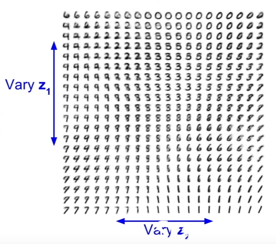
• The image below shows the output after varying the elements of z, and the different outputs it gives us when the model is trained on the MNIST dataset.

• 

• Notice how the data generated varies smoothly. This is because of our choice of the prior.
• One of the drawbacks of VAEs is that they have some blurry artifacts, unlike that given out by GANs. This is therefore still an active area of research.

In summary

• VAEs are a probabilistic spin on autoencoders enabling them to generate new images.
• VAEs define an intractable density, which we can solve by making variational approximations on the lower-bound that make them tractable. This is reason they are called “variational” auto-encoders.
• An advantage of using VAEs is that the feature representation given by the encoder can be used as a prior for other supervised learning tasks.
• Produces blurry images and lower quality compared to GANs.

Thanks for reading!