I am currently taking a course on visual learning and representation taught by Prof. Deepak Pathak. As a part of one of our assignments, we are implementing GANs from scratch. I have always been fascinated by the sort of results that GANs seemed to produce, and their working was always a blackbox. However, after reading the original whitepaper (which was beautifully and elegantly written), I am able to appreciate the simplicity of these networks even more. Here’s my take on breaking down the original 2014 paper on GANs by Ian Goodfellow et., al. This paper triggered its own line of research and today has come very far from its humble origins. However, for a paper that came out back in 2014, it still retains a lot of the modern methods and techniques used. Let’s break this paper down.
History and Introduction
- As a short historical note, in 2012, AlexNet had taken the deep learning community by storm and by 2014, people already knew how to build good image classifiers (However, ResNets had not yet taken over the community at this point).
- At this point, generative neural networks were non-existent. Prior to this, popular data generation methods included the use of auto-encoders, and their results were really blurry and had a lot of unwanted noise and artifacts.
- As a slight tangent, to recap what encoders do, have a look at the image below:
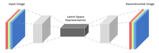
- The input image goes through a bottle-neck and is later up-sampled to get the original image back. The network is trained to match the original image as closely as possible. It has popular use-cases in image compression. An important aspect to note here is that the output is adjudged to be good or bad based on the data.
- GANs were unique in that it was the first time that the generator did not directly get feedback from the data. The key idea here was that in 2014, the research community was doing a great job building classifiers. They wanted to use the power of these classifiers (called discriminators in this context) to train a generator, without directly using the data. This is what made this work really ground-breaking and novel.
- The authors describe this relationship between the discriminator (i.e., the classifier) and the generator as a two-player zero-sum game (minimax game). What this means is that in every round, there is a clear winner and loser. Either the discriminator is able to figure out whether the image shown to it is from the dataset or from the generator (and this means the discriminator wins), or the generator is able to fool the discriminator into thinking that the image it generated is from the dataset (the discriminator loses).
- Let’s call the generator G and the discriminator D. In other words, the objective of G is to maximize the probability of D making a mistake. The architecture is like a competition between two players. This is why the paper has the name adversarial – meaning something involving conflict or opposition. In this case, the generator has an adversary, the discriminator – and each one tries to outsmart the other.
- They also say that in this representation, if G and D are distributions, there exists a unique solution. The unique solution is that G learns the distribution of the training data, and D is equal to 1/2 everywhere else. This is depicted in the image borrowed from the original paper.
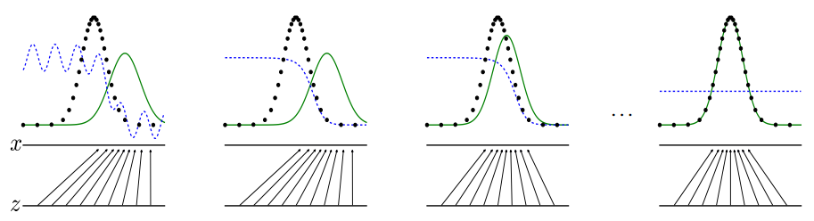
- Initially, the data (black dots), and the generator (green line) have different distributions and the discriminator is somewhat able to distinguish between them (assuming that the discriminator is non-ideal). When the discriminator is ideal, as in the second image, it is clearly able to distinguish between the data and the discriminator.
- The goal of the generator is to move its distribution in the direction of increasing gradient (up the blue dotted line). The third image shows the green line moving towards the black dotted line as indicated by the direction of increase in the gradient.
- Eventually, the generator and the discriminator are perfectly overlapped leading to the unique solution mentioned earlier. The discriminator is utterly confused at this point and is no longer able to distinguish between the data and the generated images. As a result, at all points in the space, it outputs 0.5 probability. This means that the generator has won the game.
- If G and D are both multi-layer perceptrons (a.k.a., a neural network), both models can be trained only back-propagation and dropout algorithms, which were both well-established at the time.
Loss Function and Vanishing Gradients
- As mentioned briefly earlier, both the generator and the discriminator are represented as multi-layer perceptrons (MLP).
- The generator is initialized as a uniform distribution having noise characteristics p _g (this usually refers to the mean and standard deviation). Let’s call the parameters that the multi-layer perceptron learns as \theta _g. The representation that maps the generator to the data-space is then given by G(p _g, \theta _g).
- The discriminator has MLP parameters \theta _d which outputs a single probability that x came from the generator or from the data. We train G to minimize the following logarithmic loss: log (1- D(G(z))).
- Every minimax game has a value function associated with it. In this case, the value function is given by: minmax V (G,D) = E_{x ~ p_{data} (x)} [log D(x)] + E_{z ~ p_z (z)} log (1-D(G(z)))
- The game is played in an iterative and numerical approach. Initially, when G is terrible at providing similar examples to the data, D will be able to differentiate between generated examples and the training data easily. This will mean that the term log (1-D(G(z)) will saturate and will not provide sufficient gradients for learning.
- As a result, instead of this loss, the objective of maximizing log D(G(z)) for G will be a better heuristic early on during training since it provides better gradients that do not saturate.
- During training, to make it computationally less expensive, D is trained in steps of k. There are iterations for which D is optimized k times, followed by 1 step of optimizing G. This will keep D at near optimal conditions, given that G is changing slowly.
- On a related note, this is not the same as mode collapse – a common problem in GANs where the generator produces the same conservative outputs that are likely to trick the discriminator. If the discriminator is not good enough to get out of this local minima, we will have a very boring GAN. Methods to remedy this are for another post.
The Algorithm
- The image below shows the original algorithm from the paper.
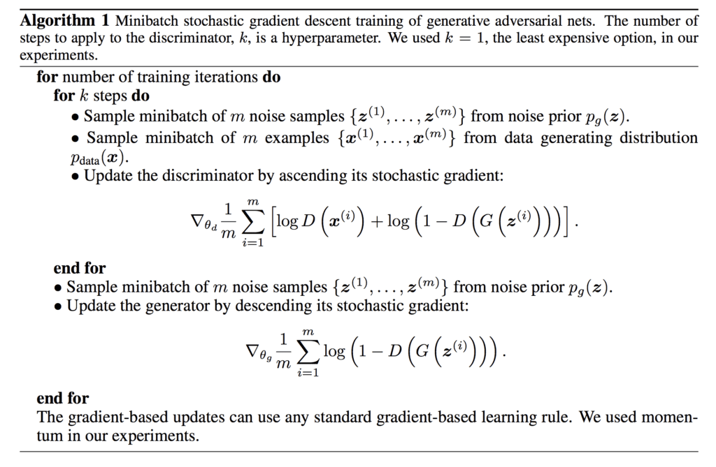
- They use k = 1 all the experiments – the least computationally expensive step.
- You first sample m batches of examples from the noise samples and the data generator. Using this sampled data, you update the discriminator by finding the gradient of the value function and moving in ascending direction of the stochastic gradient. You do this for k-steps.
- After the discriminator has been updated, you move on to update the generator. You sample m samples from the noise prior, and update the generator by descending its gradient.
Experiments
- Their implementation of generator had the following properties:
- The generator nets used a combination of ReLU and sigmoid activations.
- The discriminator used maxout activation.
- Dropout was applied in the training of the discriminator net.
- They used noise ONLY at the input. While theoretically they could have applied noise and dropouts anywhere along the network, they decided to use it at the BEGINNING only – this was another correct decision that was made along the way to nudge the probability of success of this model.
- They evaluate their model by fitting a Gaussian-Parzen window to the samples generated by G, and reporting the log-likelihood under this distribution. This method of estimating the likelihood does not perform as well in high-dimensional spaces, but was the best method available at the time. Even today, there is scope for improving the metrics used to evaluate the performance of these models.
- While GANs did not outperform similar models at the time, they were very competitive to the state-of-the-art.
- They also showed results on MNIST by interpolating in the Z-space. This is a common method used even today when showing the performance of GANs.
Advantages and Disadvantages
Compared to the approaches at the time, the advantages and disadvantages of GANs were presented as follows:
Disadvantages:
- There is no explicit representation of the probability distribution used for initializing the generator. You can only sample from it.
Advantages:
- Since this is a deterministic approach that involves using back-propagation, we don’t need Markov models (that usually model stochastic events).
- No inference is needed during training (very costly process)
- A wide variety of functions can be incorporated in the model.
The paper ended under the prescribed limit of eight pages (savage!), and also predicting major lines of work that would fill up research journals and conferences in the years to come.
I hope you enjoyed reading this as much as I enjoyed writing it!